2nd Project - Exploring Unemployment in US

Today I will make some more exploratory data analysis, on a dataset regarding unemployment statistics in USA. I will be using different approaches to answer some random questions as I don't have a specific objective.  
I will be using the September 2013 version of this this dataset, available online.
I retrieved the data from the edX course "The Analytics Edge" which I highly recommend! 

The observations in the dataset represent people surveyed in the September 2013 CPS who actually completed a survey. While the full dataset has 385 variables, in this exercise I will use a more compact version of the dataset, which has the following variables:

Variable	Description
PeopleInHousehold	Number of People in the interviewee’s household
Region	The census region where the interviewee lives
MetroAreaCode	A code that identifies the metropolitan area in which the interviewee lives (missing if the interviewee does not live in a metropolitan area)
Age	The age, in years, of the interviewee. 80 represents people aged 80-84 and 85 represents people aged 85 and higher
Married	The marriage status of the interviewee
Sex	The sex of the interviewee
Education	The maximum level of education obtained by the interviewee
Race	The Race of the interviewee
Hispanic	Wheter the interviewee is of Hispanic ethnicity
CountryOfBirthdayCode	A code identifying the country of birth of the interviewee.
Citizenship	The United States citizenship status of the interviewee
EmploymentStatus	The status of employment of the enterviewee
Industry	The industry of employment of the interviewee (only available if they are employed)

Let's start

#Installing packages
install.packages("ggplot2")
install.packages ("dplyr")
install.packages("devtools")
install_github("easyGgplot2", "kassambara")
library(ggplot2)
library("dplyr")
library(devtools)
library(easyGgplot2)

#Reading CSV file
cps=read.csv("CPSData.csv",header=T,sep=",")
str(cps)
# Set to factor once the variable is 0 if it's not Hispanic and 1 if it's Hispanic 
cps$Hispanic=as.factor(cps$Hispanic)  

#Summary statistics for metric variables
require(stargazer)
stargazer(cps, omit= c("MetroAreaCode","CountryOfBirthCode"),type="text", 
          title = "Descriptive statistics", digits=1)

#boxplot for numeric variables
par(mfrow=c(1,2))
boxplot(cps$PeopleInHousehold, xlab="People in Household")
boxplot(cps$Age, xlab="Age")

Watching to summary statistics we can see that maximum of People in households value is 15.When looking also to the boxplot, we are able to see that there are outliers (the ones presenting people in household >=8)
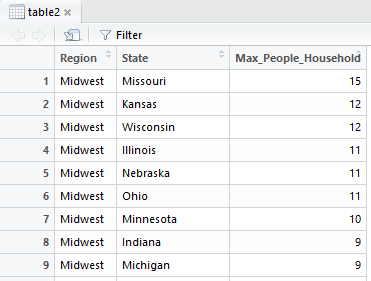
Let's discover what is maximum number of people living in Household where number of PeopleInHousehold>8  in each Region and State.
Minimum value of Age variable is 0 which is not possible. Considering that minimum age of a person to be able to answer a questionnaire is 14 years old, let's also treat this wrong values.

#from dplyr package
#Treating Age
cps$Age=ifelse(cps$Age<14,NA, cps$Age)

#Maximum number of people living in Household per Region and State
table2 = cps %>%
  filter(PeopleInHousehold>8) %>%
  group_by(Region, State) %>%
  summarise(Max_People_Household = max(PeopleInHousehold)) %>%
  arrange(Region, desc(Max_People_Household))
view(table2)

We can see the results sorted by Region and number of Maximum People in Households in descendent order.
The maximum number of people living in a Household that we can find in this dataset living in Missouri, Midwest, is 15. 

#How many interviewees are in each Region
table(cps$Region)

 We can see that the majority of interviwees are from South region

#How many interviews are Native citizens of US
table(cps$Citizenship)

 We can see that the majority of interviwees are US Native.

#What is the average age in each Region 
tapply(cps$Age, cps$Region, mean)

 In the output (which have more information than shown here), we are able to see that Utah is the youngest Region, with an average age of the interviewees of ~31 years old. On the contrary, West Virginia is the oldest Region, with an average age of the interviewees of 42,5. 

#What is the percentage of each employed status of interviewees
ggplot(data=na.omit(cps), aes(x=EmploymentStatus)) + ggtitle("Employment Status") + 
  geom_bar(aes(y = 100*(..count..)/sum(..count..)), width = 0.5, na.rm=FALSE)+ ylab("Percentage")  +coord_flip()  +theme_bw() +theme(panel.border = element_blank(), panel.grid.major = element_blank(), panel.grid.minor = element_blank())

We can see that the majority of interviewees are Employed (more than 75%).

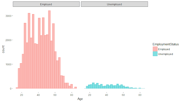
#Let's check the distribution of Age between employed and unemployed people
ggplot2.histogram(data=na.omit(subset(cps,EmploymentStatus=="Employed"|EmploymentStatus=="Unemployed")), xName='Age',groupName='EmploymentStatus', legendPosition="top",faceting=TRUE, facetingVarNames="EmploymentStatus",facetingDirection="horizontal")+theme_bw()+ theme(panel.border = element_blank(), panel.grid.major = element_blank(), panel.grid.minor = element_blank())

The majority of Employees are between 40 and 60 years old. Again, is very easy to understand in this plot that the amount of employed people is much higher than unemployed. Here we are not able to see in a very clear way the distribution of unemployed people. We could do separate histograms and change the axis options if needed.

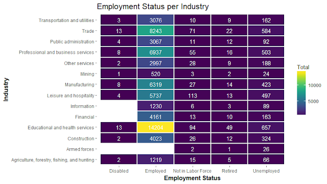
# What is the distribution of Employed Status per Industry
require(ggthemes)
require(viridis)
Employed_count = cps %>% group_by(EmploymentStatus,Industry)%>%   summarise(Total = n())
Employed_count$EmploymentStatus = ordered(Employed_count$EmploymentStatus)
ggplot(na.omit(Employed_count), aes(EmploymentStatus, Industry, fill = Total)) +
  geom_tile(size = 1, color = "white") +
  scale_fill_viridis()  +
  geom_text(aes(label=Total), color='white') +
  ggtitle("Employment Status per Industry") +
  xlab('Employment Status') +theme_bw()+ theme(plot.title = element_text(size = 16), 
   axis.title = element_text(size = 12, face = "bold"))  + theme(panel.border = element_blank(),        panel.grid.major = element_blank(), panel.grid.minor = element_blank())

Educational and health services is the industry where we have more employed interviewees. On the other hand, there are no employees in Armed forces.