6th Project - Decision Tree

Today's project is about building a decision tree in a retail dataset with the core business of selling Wines (also on online channel). In order to understand what drives the decision of a customer to buy a Large Wine Rack of 100$ (target variable LGRack),and to build a model capable of predicting which customers have higher probability of buying the accessory, I will use a classification tree algorithm. I will start with an exploratory data analysis with a package I found really helpfull specially for the analysis I will perform today. The description of the dataset is below:

#Intalling Packages
install.packages("SmartEDA") #For Exploratory data analysis
library("SmartEDA")

#Read dataset
data=read.csv("Book1.csv",head=T, sep=";")

#Data preprocessing - Set binary variables as factors (including CustID since this will not be used in any analysis)
data$Custid=as.factor(data$Custid)
data$Kidhome=as.factor(data$Kidhome)
data$Teenhome=as.factor(data$Teenhome)
data$SMRack=as.factor(data$SMRack)
data$LGRack=as.factor(data$LGRack)
data$Humid=as.factor(data$Humid)
data$Spcork=as.factor(data$Spcork)
data$Bucket=as.factor(data$Bucket)
data$Access=as.factor(data$Access)

#First table information
ExpData(data=data,type=1,DV=NULL)

We can see that the dataset has 10.000 observations, 26 variables (17 are numeric and 9 are factor variables). We can also see that there are no missing values in this dataset. Let's now look at some statistics. What is good in this package is the ability of producing summary statistics and visualization considering our target variable in study (in this case LGRack):

#Summary statistics for continuous variables
stat=ExpNumStat(data,by=c("GA"),gp="LGRack",Qnt=NULL,MesofShape=2,Outlier=FALSE,round=3)
#to exclude some information provided in the summary table of ExpNumStat() function that I don't want to visualize.
stat=stat[,-c(4,5,6,7,8,9,10,17)] 

In the output table presented here, I didn't include all variables (because it's a large table) but we can see here some statistics like minimum, maximum, mean, media, standard deviation and so on for each variable (All) and also for the cases when customers bought LGRack (LGRack:1) and when customers didn't buy the LGRack (LGRack:0). When looking to this summary statistics, we are able to check if there are strange values that might be errors: for example in Age variable, in some datasets i previously analysed, I found customers with 99 years old which was of course an error. In this dataset, I didn't find any strange values, except for the Web visits and Webpurchases minimum value: In webvisit variable, minimum value is 0 which means that in the dataset we have customer(s) that didn't visit the website. Well if that's the case, then we should also have in WebPurchase variable (% purchases made in website) 0 as minimum value. Let's further analyse this customers:
#Analysing customers with webvisits=0
stat_webpurch=ExpNumStat(subset(data,WebVisit==0),by=c("A"),Qnt=NULL,MesofShape=2,Outlier=FALSE,round=3)
stat_webpurch=stat_webpurch[,-c(4,5,6,7,8,9,10,17)]

We can see that customers that have no vistis to the site (Webvisit=0) have minimum value of Webpurchase variable = 5, which does not make sense. So I will exclude this 32 customers from the dataset.
#Excluding customers with Webvisit <=0
data=subset(data,WebVisit>0)

Let's now do some visualization:
####Visualization###
#Barplots for categorical variables
ExpCatViz(data,gp=NULL,fname=NULL,clim=10,margin=2,Page = c(3,3))

We can see that in what concerns LGRack, the majority of the customers didn't buy it (93%). The same trend with the other accessories is seen, since in every variable we can see that the higher percentage corresponds to "customer didn't buy". In webvisits, we can see that the majority of customers visted the website on average 7 times per month. 

#Continuous variables taking into account target variable

ExpNumViz(data,gp="LGRack",type=1,nlim=NULL,fname=NULL,col=c("pink","yellow","orange"),Page=c(3,3))

From the output we can see that customers who bought the LGRack have higher income, higher monetary value, are elder, and also more frequent customers. We are also able to see that in some variables we have outliers, like on Income, Monetary,Frquency,  LTV, Recency and Perdeal.

Now that we have made some exploratory analysis (this is not the core of the post so I didn't get deep on this topic), let's build our tree, after excluding from the analysis the other categorical variables and after changing the variables which are represented in percentages % to absolute value:

#Exlude categorical variables (except LGRack) from dataset

data=data[,-c(1,6,7,21,23,24,25,26)]

#Change variables

  for(i in 9:16){

  data[,i]=(data$Monetary*data[,i])/100

}

Because our target variable (LGRack) is binary (0=not bought, 1=bought), we will build a classification tree. Let us now see how to construct the classification tree in R. The significance of the sample used to obtain the model is essential to have a minimum of guarantees of the representativeness of the model constructed. So it makes no sense to get a decision tree using half a dozen examples of decisions. In fact, the larger the sample used the better. Before we start, we should think on a question:

What confidence can we have in the performance of the model we are about to build?

One of the most practical ways of responding to this question is to test the model using new cases of customer decisions (bought or not bought), and to account for the incorrect decisions, when compared with the customer decisions made (predicted) by the decision tree.
One way to simulate the existence of more cases to test our model is to divide the cases that we have into two sub-sets: one to obtain the model; and another to test it. Let's see how to do this in R:
# total number of rows in the data frame
n <- nrow(data)
# number of rows for the training set (80% of the dataset)
n_train <- round(0.80 * n)
# create a vector of indices which is an 80% random sample
set.seed(123) # set a random seed for reproducibility 
train_indices <- sample(1:n, n_train)
# subset the data frame to training indices only
train <- data[train_indices, ]
# exclude the training indices to create the test set
test <- data[-train_indices, ]

Okay, so now we are ready to start building our decision tree: 
#Installing packages
library(rpart)
#Creating the tree in the training dataset: method="class" specifies this is a classification tree
data_model <- rpart(formula = LGRack ~.,data = train,method = "class")
data_model

After obtaining the tree we asked R to show the content of the object to which we attribute the result. R presents the decision tree as text. As we shall see later, it will also be possible to obtain a graphical representation. Let us now analyze the information given by R on the tree object. 

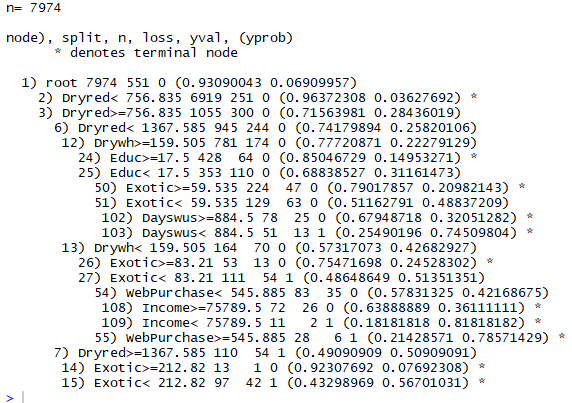
First, the R tells us the number of cases used to obtain the model. Next, a series of lines representing the different tests and nodes of the tree are presented. These are presented following a certain indentation and with an associated number, in order to better understand the hierarchy of the tests. Higher indentation means that the test / node is situated at a lower level in the tree. Thus, in this concrete example the first line identified with the number 1 gives us the information concerning the root node of the tree, before performing any test on a variable.

According to this information, we can see in the root node, that before we know / test the value of any variable, the best decision would be "0" (i.e. "not bought"). This decision is supported by the fact that of the 7974 examples given to R only 551 are of class "1=bought" which leads to a probability of 93% of any customer being a case of "not bought", and a 6.9% probability of being a case of  "bought". These probabilities are the numbers presented in parentheses. From this root node we have two derivations depending on the value of the Dryred variable. These derivations are identified by numbers 2 and 3, and correspond to the next level of indentation.

Of the 7974 cases provided to R, 6919 customers have Dryred monetary value <756$ and in these, the majority class is "not bought", only 251 correspond to situations where customer bought the LGRack. If the customer has Dryred monetary value <756$ than a decision is reached (the R indicates this by placing a "* " on the line), which in this case is not bought (the probability of a customer to not buy the LGRack is 96%)
In summary, using the numbers and indentation, you can get an idea of the shape of the decision model obtained with the rpart function.

Let's now visualize the tree:
#Plotting tree
install.packages("rpart.plot")
library(rpart.plot)
boxcols <- c("pink", "palegreen3")[data_model$frame$yval]
par(xpd=TRUE)
prp(data_model, faclen=0, cex=.6, extra=5, box.col=boxcols)

We can conclude that customers that buy more than 757$ and less then 1368$ in DryRed wines, that spend more than 160$ in dry white wines, that have spent more then 83$ in uncommon wines (exotic), that spend less then 546$ in web purchases and that have an income > 76.000$ have the higher probability of buying the LGRack (82%).

Now we can obtain the tree predictions for the separate sample cases of testing:
#Predicting LGRack for test data
class_prediction <- predict(object = data_model, # model object
                            newdata = test, # test dataset
                            type = "class") # return classification labels

These predictions can now be compared to the true values of the test cases and thus get an idea of tree performance:
# calculate the confusion matrix for the test set
library(caret)
confusionMatrix(data = class_prediction, # predicted classes
                     reference = test$LGRack) # actual classes

In this particular case, we are comparing the row values (tree predictions) with the customer decision on test cases ("real" values). The resulting information is commonly known as the confusion matrix of the model predictions. She tells us that of the 1851(1831+20) cases in which customers didn't buy the LGRack, the tree also predicted the same outcome in 1831 cases, but made the wrong prediction in 20 cases. On the other hand, of the 42 cases in which customer bought the LGRack, the tree said the same to 22 of them, but predicted wrongly for 20 cases. With this information it is easy to calculate the percentage of wrong decisions of the tree, if we calculate the confusion matrix with table() function, since the result of the table function is an array.The percentage of wrong decisions corresponds to adding all the numbers of the matrix that are not diagonal (because these are the right decisions), and divide this sum by the sum total of all numbers (which in fact is the total number of decisions made).

conf <- table(test$LGRack,class_prediction)
error_rate <- 100 * (conf[1,2]+conf[2,1]) / sum(conf)
error_rate

On the other hand, the accuracy of the tree is given by:
#Accuracy:
acc=sum(test$LGRack==class_prediction)/length(class_prediction)

We built a classification tree that presents a high accuracy and that can help the company make decisions of which customers receive for example campaigns to make them purchase the LGRack. Is important to notice that R have other functions to build classification trees, with different algorithms that take into account different metrics for classification so it would be a good approach to build the model with different algorithms and check if the accuracy increases!