
In my last post, I performed a factor analysis on the SFO passangers dataset to find underlying dimensions of respondents satisfaction. Just to recap, here are the 4 dimensions found in FA:
Factor 1 - Internal Services
Factor 2 - Cleanless services
Factor 3 - External services
Factor 4 - Entretainment services
In this post, my objective is to perform a cluster analysis to segment the passengers in homogenous groups based on their satisfaction dimensions and characterize them based on sociodemographic variables, using a hierarchical clustering method. To better understand what is Hierarchical clustering, I will post below the explanaition I found in https://www.r-bloggers.com/how-to-perform-hierarchical-clustering-using-r/ with some comments/edits from my side. What is Hierarchical Clustering?
Clustering is a technique to join similar data points into one group and separate out dissimilar observations into different groups or clusters. In Hierarchical Clustering, clusters are created such that they have a predetermined ordering i.e. a hierarchy. For example, consider the concept hierarchy of a library. A library has many sections, each section would have many books, and the books would be grouped according to their subject, let’s say. This forms a hierarchy.
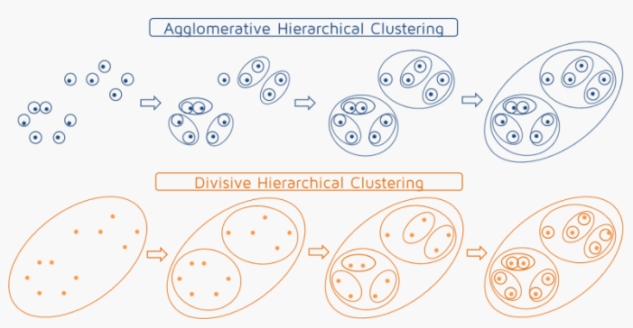
In Hierarchical Clustering, this hierarchy of clusters can either be created from top to bottom, or vice-versa. Hence, it’s two types namely – Divisive and Agglomerative. Let’s discuss it in detail.
In Hierarchical Clustering, this hierarchy of clusters can either be created from top to bottom, or vice-versa. Hence, it’s two types namely – Divisive and Agglomerative. Let’s discuss it in detail.
Divisive Method
In Divisive method we assume that all of the observations belong to a single cluster and then divide the cluster into two least similar clusters. This is repeated recursively on each cluster until there is one cluster for each observation. This technique is also called DIANA, which is an acronym for Divisive Analysis.
Agglomerative Method
It’s also known as Hierarchical Agglomerative Clustering (HAC) or AGNES (acronym for Agglomerative Nesting). In this method, each observation is assigned to its own cluster. Then, the similarity (or distance) between each of the clusters is computed and the two most similar clusters are merged into one. Finally, steps 2 and 3 are repeated until there is only one cluster left."
Please note that Divisive method is good for identifying large clusters while Agglomerative method is good for identifying small clusters.HAC’s account for the majority of hierarchical clustering algorithms while Divisive methods are rarely used.
I will proceed with Agglomerative Clustering, but first, let me briefly explain how hierarquical clustering works:
HAC Algorithm
Given a set of N items to be clustered (in our case the passengers), and an NxN distance (or similarity) matrix, the basic process of Johnson’s (1967) hierarchical clustering is:
- Assign each item to its own cluster, so that if you have N items (passengers), you now have N clusters, each containing just one item. Let the distances (similarities) between the clusters equal the distances (similarities) between the items they contain.
- Find the closest (most similar) pair of clusters and merge them into a single cluster, so that now you have one less cluster.
- Compute distances (similarities) between the new cluster and each of the old clusters.
- Repeat steps 2 and 3 until all items are clustered into a single cluster of size N.
In Steps 2 and 3 here, the algorithm talks about finding similarity among clusters. So, before any clustering is performed, it is required to determine the distance matrix that specifies the distance between each data point using some distance function (Euclidean, Manhattan, Minkowski, etc.). Just to give you a better understanding of how this is calculated, I'll give you the example: To calculate de euclidian distance between passenger 1 of dataset and passenger 2 in what concerns Factor 1 (X), Factor 2 (Y), Factor 3 (Z), and Factor 4 (P), the formula, using Euclidian Distance is as following:

At this stage, we selected how to compute the distance between the objects (passengers) when they are theirself a cluster, but in successive steps they will jointly become a cluster with more than 1 passenger, so we have to decide now the criterion for determining which clusters should merge at successive steps, which means, the hierarchical clustering algorithm to use. Again, there are several algorithms such as "Complete", "Ward", "Single", etc:
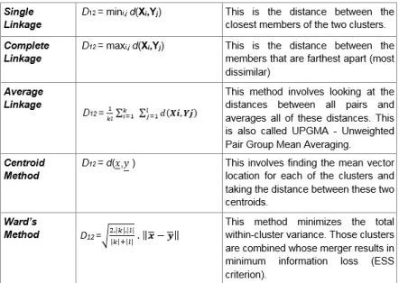
Because we can not say that a specific method is the best one, the best approach is to perform the analysis with all methods and choose the one that is more interpretable (which gives the best solution). In this analysis, I will perform the analysis with the 5 methods and I will plot the so well known "Dendogram", the common graphic used in hierarchical clustering to plot the solution.
To perform clustering, the data should be prepared as per the following guidelines:
- Rows should contain observations (or data points) and columns should be variables (in our case, the variables will be the factors - dimensions that explain the latent variables of satisfaction
- Check if your data has any missing values, if yes, remove or impute them.
- Data across columns must be standardized or scaled, to make the variables comparable (if they are in different scales - in our case this step is not necessary since we will be using the scores of the factors)
components=factor_analysis$scores
data=cbind(airport, components)
#With the following command, I will get for each par of passengers (scores) the distances in what regards the factors (euclidian distance)
d <- dist(components, method = "euclidean")
# Hierarchical clustering with agglomerative algorithm
hc1 <- hclust(d, method = "complete" )
hc2 <- hclust(d, method = "ward" )
hc3 <- hclust(d, method = "single" )
hc4 <- hclust(d, method = "average" )
hc5 <- hclust(d, method = "centroid" )
# Plot the obtained dendrograms
par(mfrow=c(2,3))
plot(hc1, cex = 0.6, hang = -1)
plot(hc2, cex = 0.6, hang = -1)
plot(hc3, cex = 0.6, hang = -1)
plot(hc4, cex = 0.6, hang = -1)
plot(hc5, cex = 0.6, hang = -1)

Whe can see in the output that only "Ward" method produces an interpretable solution, so I will continue with this one as the algorithm method chosen. To decide what is the best number of clusters to final solution, we can draw a line where there's a big "jump" in the dendogram (i.e. where the successiv differences between the distances increase suddenly). For instance, we can clearly see that the first biggest jump would make 4 clusters:
#Dendogram
par(mfrow=c(1,1))
plot(hc2, cex = 0.6, hang = -1)
rect.hclust(hc2, k = 4, border = 2:5)

clusters=cutree(hc2, k = 4)
data=cbind(data, clusters)
install.packages ("dplyr")
library(dplyr)
summary_table = data %>%
group_by(clusters) %>%
summarise(services = mean(RC4), information=mean(RC1), external_services=mean(RC3),Cleanless=mean(RC2), count=length(RESPNUM))

Finally, I will export the dataset to excel to create pivot tables with Demographic variables to end with the characterization of clusters!
#Write CSV
write.csv(data,file="factor.csv")

Cluster 1(n=951) -
Group of passengers that on average is more satisfied with services (internal and external) then with information provided and cleanless. This cluster has more a less the same number of women and men, and the majority of passengers in this cluster have between 25-34 years old, though this is also the group where we have a high percentage of old people (12,83%). This is a cluster with the passengers that present a high income.
Cluster 2(n=694)
Group of passengers that on average is more satisfied with information provided in the airport then with services (internal and external) and cleanless. The majority of passengers in this cluster are men and are middle age people. In line with the first cluster, the majority of passangers of group 2 have an anual income of over 150,000$.
Cluster 3(n=591)
Group of customers that on average is more satisfied with internal services, information provided in the airport and cleanless then with external services. The majority of passangers of this cluster are women and again middle age and such as cluster 1, we find a high percentage of older people (12,69%). This group of passengers have an anual income between 50,000$ and 100,000$.
Cluster 4 (n=595)
Group of customers that on average is more satisfied with external services and cleanless then with internal services and information. Such as cluster 1, this group have more a less the same percentage of women and men, and it is where we find a high percentage of young people (between 18 and 24). They have also a high anual income.
Based now on the output, we could set specific actions to adress the necessities of each group, but for that we would need to get a further analysis to understand why the customers are unhappy with the different services. Also, in the beggining of the study I dropped the "Overall satisfaction" variable which would be interesting to have now.


Really nice blog post.provided a helpful information.I hope that you will post more updates like this
ReplyDeleteData Science online Course Bangalore